GroupWAR
Every few years Canada picks a hockey team for a best-on-best tournament, and every few years the country argues about it. The argument is usually about individual players: who had the better season, who deserves the spot. But a national team is a group. Eighteen skaters have to fit together, and the eighteen best individuals are not automatically the best eighteen.
Jaden and I wanted to see what happens if you treat the roster as a single object and search for it. Score any candidate roster with a learned model, test it against an opponent that is trying to beat it, and look for the roster that holds up. We called the project groupWAR, after the roster-level version of wins above replacement that falls out of it. We ran it on Canada for the 2025 4 Nations Face-Off, and on USA and Canada basketball for the 2024 Paris Olympics.
Scoring a roster
The scorer is a graph convolutional network. Each player is a node, and edges are weighted by how much time two players have shared on the ice or court, so the model can pick up relationships through common teammates as well as direct ones. It has six layers with a hidden size of 128. A DeepSet layer then summarizes each side into one lineup embedding, which makes the order you list players in irrelevant.
The output head is antisymmetric: $f(H, A) = 1 - f(A, H)$. If home beats away with probability 0.6, away beats home with probability 0.4. That sounds obvious, but a network will not do it on its own, and without it home advantage leaks into the learned features. The training target is $y = \sigma(\Delta / 10)$, where $\Delta$ is the goal or point differential, and we trained an ensemble over six cross-validation folds and averaged the predictions.
Hockey used NHL play-by-play, shift and boxscore data for 2021-22 through 2025-26, with each player-season as a 14-dimensional feature vector (shot and attempt rates, xG, zone starts, TOI, size, position). Basketball came from a public Kaggle SQLite dump. We started with two seasons, about 2,400 games, and later expanded to 2019-20 through 2023-24, about 6,100 games, with 23 features per player including a 7-zone shot breakdown and zone-aware assist rates.
We also fit a ridge-regression adjusted plus-minus for every player, and deliberately kept it out of the network. It is used only to rank players and order rotations. Keeping it separate meant we could check it against public RAPM without grading our own homework. Across 287 matched players it came out at Pearson $r = 0.81$ and Spearman $\rho = 0.78$, with 38 of our top 50 also in the public top 50.
Testing a roster against someone trying to beat it
A roster that wins against a passive opponent is easy to find. We wanted one that wins when the other side reacts. So each candidate is evaluated as a leader-follower game. The leader (our roster) adjusts how its players are deployed together; the follower (the opponent) adjusts its own deployment and the matchups to push our win probability down. Both sides take 100 gradient steps, with the leader updating five times for every follower update. Player features stay fixed. Only the interaction graph changes, and it gets projected back after each step so neither side can win by just scaling every edge up.
The opponent set was a practical compromise. Hockey played against USA plus Edmonton and Florida as proxy opponents, because we had rich NHL lineup data and very little for Sweden, Finland or Czechia. Basketball USA played Canada, France and OKC; Canada played USA, France and OKC.
This framing has a bias we wrote about in the paper. A worst-case opponent punishes any single exploitable weakness, so the score prefers balanced rosters over high-ceiling ones. Real tournament coaches have a few days of prep, not 100 gradient steps.
Searching the space
The number of possible rosters is enormous, and each evaluation runs a small adversarial optimization, so exhaustive search was never on the table. We locked in the players no coach would leave off (McDavid, MacKinnon, Crosby, Makar and Theodore for hockey; Curry, LeBron, Durant and Davis for USA; SGA and Murray for Canada), which takes them out of the search and spends the budget on the depth spots.
The search then runs in two phases. A tournament phase forms random teams from the eligible pool, keeps the top third intact, and strips the lowest-usage players from the rest, until about twice the target size remains. A greedy phase then tries every single swap between a roster spot and a bench candidate, scores them all in one batched pass, and takes the best one until nothing improves.
None of this guarantees a global optimum. It makes an expensive score tractable, which is all we needed.
The first hockey run was ten centers
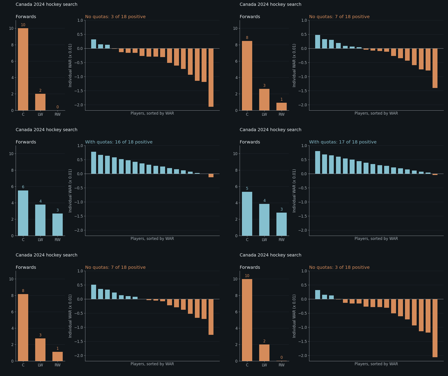
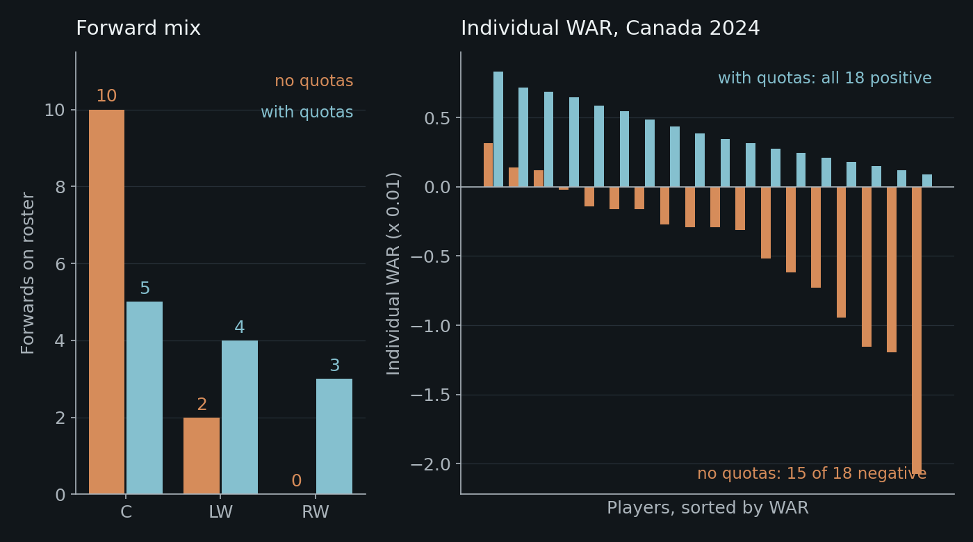
Our first serious hockey run, a diagnostic on Canada 2024 with no position rules, converged to 10 centers, 2 left wings and 0 right wings. Its team score was 0.4562, and 15 of its 18 players had negative WAR. McDavid came out at $-0.009$.
That WAR is a knockout measure: replace one player with a placeholder vector and see how much the team score drops.
$$\text{WAR}_i = \hat{y}(\text{full}) - \hat{y}(\text{lineup} \setminus i)$$
Negative WAR means the model likes the roster better with that player gone. McDavid being negative did not mean McDavid is bad. It meant the roster was so incoherent that removing anyone looked like an improvement. The model had never seen a team of ten centers in training, so it had no reason to score one badly.
The fix was boring. We added position quotas: at least 3 left wings, at least 3 right wings, at most 5 centers, and a six-defenseman target. The score dropped to 0.4428, and every player's WAR turned positive, from +0.0009 up to +0.0082. A 0.013 drop in score was the cost of a roster a coach would actually accept. I think that run taught me more than any of the good ones. The search had found exactly what we asked for, and what we asked for was wrong.
Summing the knockouts gives the roster-level number the project is named after:
$$\text{GroupWAR}(R) = \sum_{i \in R} \text{WAR}_i(R) = n\,\hat{y}(R) - \sum_{i \in R} \hat{y}(R \setminus i)$$
A high GroupWAR roster has no passengers. Every player's removal would cost the team something, under the same roster and the same opponents.
Canada 2025
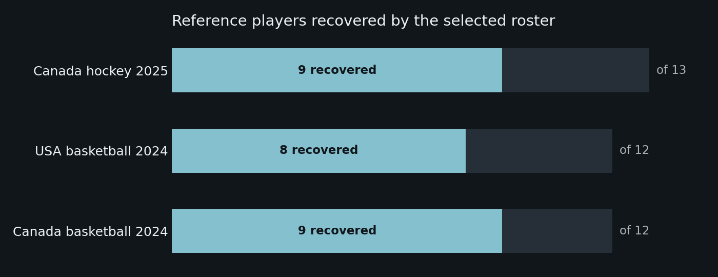
With a looser version of the quotas, the 4 Nations run finished with a score of 0.4495 and all 18 skaters positive. Before running it we wrote down a 13-player reference set of the obvious core. The roster recovered 9 of them: McDavid, MacKinnon, Crosby, Makar, Theodore, Doughty, Parayko, Stone and Reinhart. It left out Bennett, Marchand, Marner and Point.
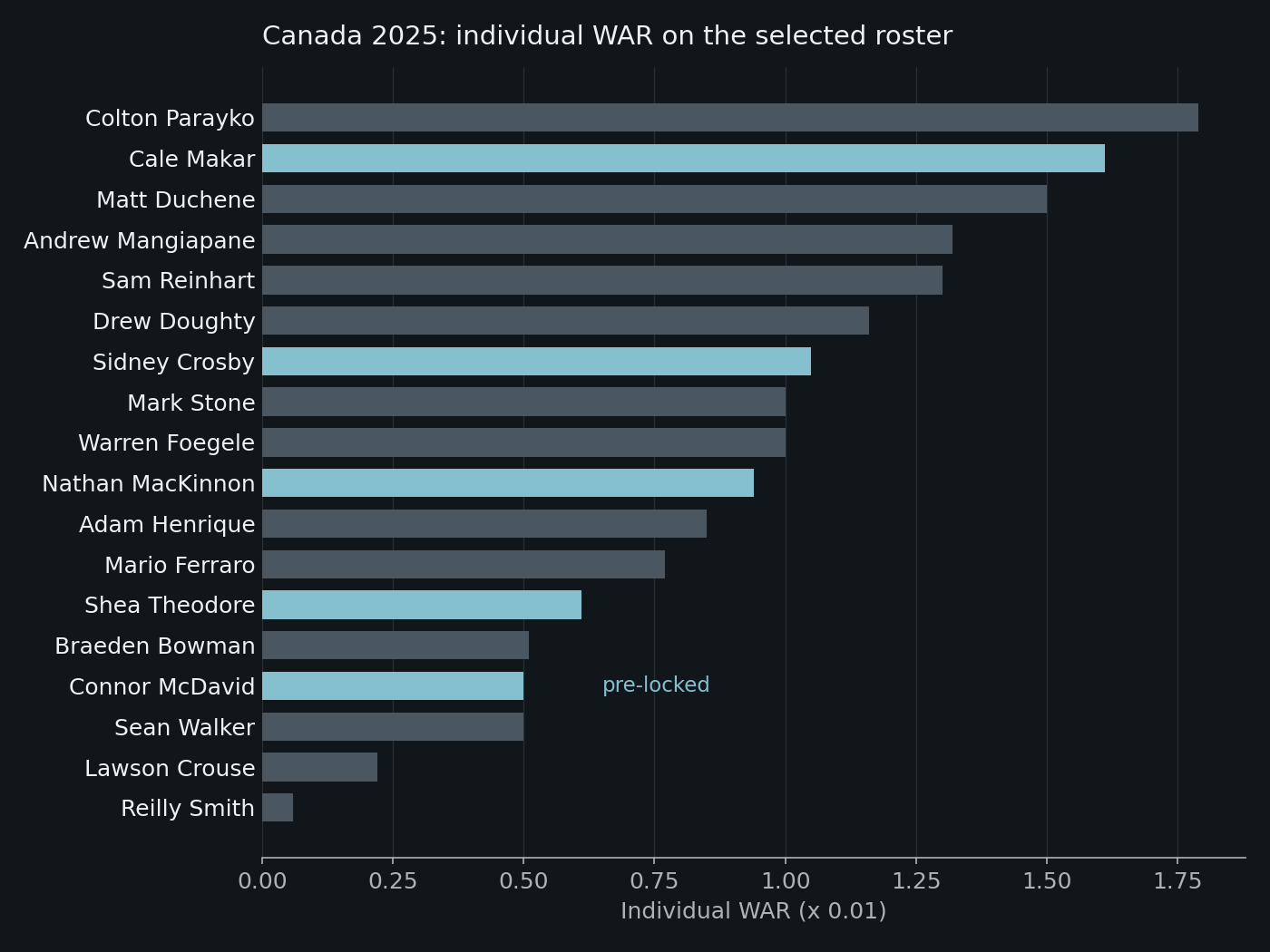
The depth picks are where the model shows its training data. Mangiapane over Marner. Foegele, Henrique, Ferraro. These are two-way regular-season role players, and a model trained on regular-season games has learned to reward exactly that. It has never watched three Hall of Fame centers play together, so it cannot know that stacking them is the point.
The Sean Monahan case is my favourite result. Ranked over the whole eligible pool, his WAR was second, behind only Parayko and ahead of MacKinnon, Makar and Point. He did not make the team, because the center quota was already full. Being the franchise center in Columbus is real information, and the model picks it up. It still does not make him a top-three center for a team with McDavid, MacKinnon and Crosby. The pipeline puts that trade-off on the table instead of hiding it inside one number.
Basketball needed a different fix
Hockey dresses 18 skaters, so an 18-a-side graph matches the decision. Basketball does not. The network scores 5 on 5, and a roster is 12. Our first workaround scored the top five against the opponent's top five and the next five against their next five, weighted 0.6 and 0.4. That baked in a starter and bench split no coach actually uses.
The version we reported uses stochastic rotation scoring. Rank the 12 by APM, build 10 overlapping five-man lineups from a fixed template (starters, two stagger units, bench-heavy units, closing units), score each one adversarially against all three opponents, and blend by weight.
| Rotation | APM ranks | Weight |
|---|---|---|
| Starters | 1, 2, 3, 4, 5 | 0.40 |
| Stagger A | 1, 2, 6, 7, 8 | 0.12 |
| Stagger B | 3, 4, 5, 6, 9 | 0.12 |
| Bench-heavy A | 2, 6, 7, 8, 10 | 0.09 |
| Bench-heavy B | 3, 6, 8, 9, 11 | 0.07 |
| Deep bench mix | 1, 9, 10, 11, 12 | 0.05 |
| Closing defensive | 1, 3, 4, 7, 8 | 0.04 |
| Big-wing mix | 2, 4, 5, 8, 11 | 0.04 |
| Guard-pressure mix | 1, 3, 6, 10, 12 | 0.04 |
| Closing shooting | 1, 2, 4, 6, 9 | 0.03 |
USA overlapped with 8 of the 12 Paris Olympians, and Canada with 9 of 12. The interesting USA decision was Joel Embiid. The tournament phase picked him, and the first greedy swap replaced him with Draymond Green. Embiid improved the starting five by +0.010 but cost the bench rotations $-0.027$, because paint-heavy second units are easy to beat with spacing. Under adversarial scoring the opponent always gets to choose that exploit. Jrue Holiday went the other way: never locked, picked in every greedy iteration, slightly worse than Lillard in the starting five and much better in the bench units.
| Case | Score | Reference overlap | All WAR positive |
|---|---|---|---|
| Canada hockey 2025 | 0.4495 | 9 of 13 | yes |
| Canada hockey 2024, no quotas | 0.4562 | not claimed | no (15 of 18 negative) |
| Canada hockey 2024, quotas | 0.4428 | not claimed | yes |
| USA basketball 2024 | 0.7418 | 8 of 12 | yes |
| Canada basketball 2024 | 0.6587 | 9 of 12 | yes |
What WAR is and isn't
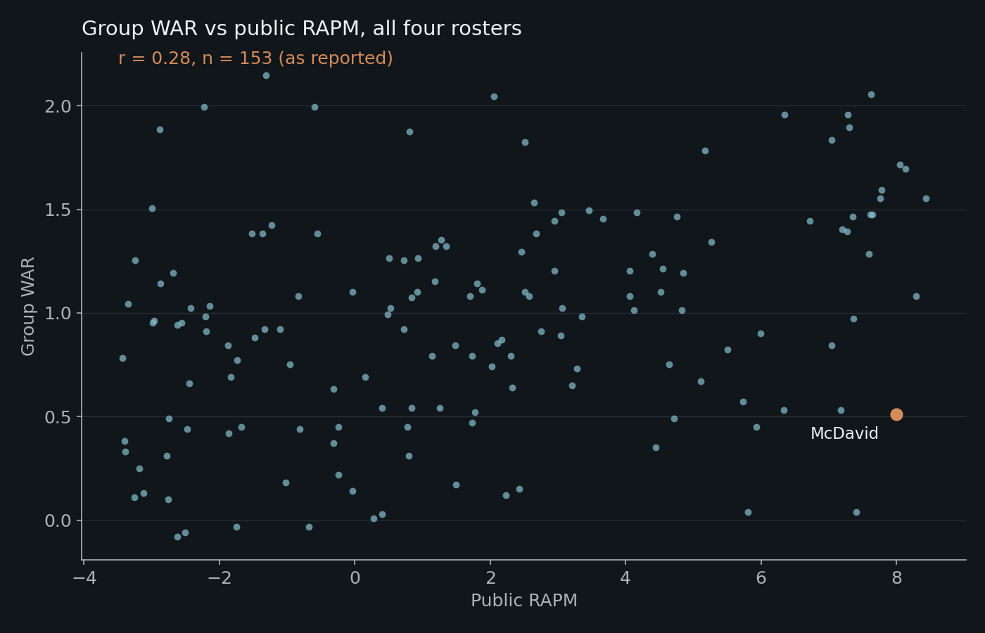
We checked individual WAR against public RAPM across 153 players from all four rosters and got $r = 0.28$. That is low, and we expected it to be. WAR here is conditional on everything else: the roster, the opponents, the model. An elite player on a star-heavy team can look replaceable, and a versatile depth player can look essential. Saying Makar is worth +0.016 only means something for that specific Canadian roster.
The larger limitation is the training data. Every game the model learned from was a regular-season NHL or NBA game. International rosters live somewhere the model has never been. The three-year averaged hockey features have a smaller version of the same problem: they flatten a breakout season like Reinhart's 2023-24 back toward his career average.